The Billion Data Point Challenge: Building a Query Engine for High Cardinality Time Series Data

Uber, like most large technology companies, relies extensively on metrics to effectively monitor its entire stack. From low-level system metrics, such as memory utilization of a host, to high-level business metrics, including the number of Uber Eats orders in a particular city, they allow our engineers to gain insight into how our services are operating on a daily basis.

As our dimensionality and usage of metrics increases, common solutions like Prometheus and Graphite become difficult to manage and sometimes cease to work. Due to a lack of available solutions, we decided to build an in-house, open source metrics platform, named M3, that could handle the scale of our metrics.

A major component of the M3 platform is its query engine, which we built from the ground up and have been using internally for several years. As of November 2018, our metrics query engine handles around 2,500 queries per second (Figure 1), about 8.5 billion data points per second (Figure 2), and approximately 35 Gbps (Figure 3). These numbers have been constantly trending upwards at a rate much higher than Uber’s organic growth due to the increased adoption of metrics across various parts of our stack.

In this article, we present the challenges we faced in designing a query engine for M3 that was performant and scalable enough to support the computation of a large amount of data every second, as well as flexible enough to support multiple query languages.

An M3 query goes through three phases: parsing, execution, and data retrieval. The query parsing and execution components work together as part of a common query service, and retrieval is done through a thin wrapper over the storage nodes, as depicted in Figure 4, below:

To support multiple query languages, we designed a directed acyclic graph (DAG) format that both the M3 Query Language (M3QL) and the Prometheus Query Language (PromQL) can be compiled to. The DAG can be understood as an abstract representation of the query that needs to be executed. This design makes it easy to add new query languages by decoupling the language parsing from the query execution. Before scheduling the DAG for execution, we use a rate limiter and authorizer to ensure only authorized users can issue requests, rate limiting them to prevent abuse.

The execution phase keeps track of all the running queries and their resource consumption. It may reject or cancel a query that results in any resource exhaustion, such as the total available memory for the process. Once a query has started executing, the execution engine fetches the required data and then executes any specified functions. The execution phase is decoupled from the storage, allowing us to easily add support for other storage backends.

While M3DB, Uber’s open source time series database, is currently the only supported storage backend for M3, in the future we plan to add support for more storage providers, such as OpenTSDB and MetricTank.

As more and more teams at Uber began using M3, tools were built on top of the platform to perform functions like anomaly detection, resource estimation, and alerting. We soon realized that we needed to place limits on our query sizes to prevent expensive queries from using up all of our service’s memory. For example, our initial memory limit for a single query was 3.5 GB, a size that enabled us to serve a reasonable amount of traffic without massively over-provisioning our system. Still, if a query host received multiple large queries, it would overload and run out of memory.

Moreover, we realized that once our query service started to degrade, users would continuously refresh their dashboards because the queries were returning too slowly or not at all. This would compound the issue by generating additional queries that would begin to pile up because the original queries were never canceled. Furthermore, we found that some power users and platforms built on top of the query service were pushing these memory limits, forcing us to think about ways to improve the system’s memory utilization.

During query execution, we spent a lot of time allocating massive slices that could store the computation results. As a result, we started pooling objects such as series and tags, a move that caused a noticeable reduction in the garbage collection overhead.

On top of that, we had assumed that our goroutine creation would be extremely lightweight, and it was, but only because every new goroutine starts with a small, 2 kibibytes (KiB) stack of memory. All of our flame graphs indicated that a lot of time was being spent growing our stack of newly created goroutines (runtime.morestack, runtime.newstack). We realized this was occurring because many of our stack calls exceeded the 2 KiB limit, and so the Go runtime was spending a lot of time allocating new 2 KiB goroutines, and then immediately throwing them away and copying the stack onto a larger 4 or 8 KiB stack. We decided we could avoid all of these allocations entirely by pooling our goroutines and re-using them via a worker pool.

Looking at usage statistics for the query service, we identified a consistent pattern in which the query service was spending a lot of time executing queries that were no longer needed, or had been superseded by a new query. This can happen when a user refreshes their dashboard in Grafana, and occurs more frequently with large, slow queries. In such situations, the service wastes resources to unnecessarily evaluate a long-running query. To remedy this, we added a notifier to detect when the client has disconnected and canceled remaining executions across the different layers of the query service through context propagation.

Although all of the above approaches reduced the query engine’s memory footprint significantly, memory utilization remained the primary bottleneck for query execution.

We knew that if we were going to support an order of magnitude increase in the scale of our query service, we would need a fundamental paradigm shift. We designed a full MapReduce-style framework for the system with separate query and execution nodes. The idea behind this design choice was that in order to ensure that the execution nodes could scale infinitely, we needed to break the query into smaller execution units (Map phase). Once the execution units were processed, we could re-combine the results (Reduce phase).

As we began to implement our design, we quickly realized the complexity of this solution, so began looking for simpler solutions.

One key insight from our evaluation process was that we shouldn’t decompress data on fetch if we are dealing with storage backends that keep data compressed internally, which is exactly how M3DB stores data. If we delay the decompression as long as possible, we might be able to reduce our memory footprint. To achieve this, we decided to take a page out of the functional programming book and redesign our query engine to evaluate functions in a lazy manner, delaying allocations of intermediary representations (and sometimes eliminating them entirely) for as long as possible.

Figure 5, above, demonstrates a linear operation – clamp_min followed by sum. During evaluation, we determined that there were two approaches to execute on this decompression: apply both functions sequentially (Approach 1) or apply clamp_min and sum to one column at a time (Approach 2). The above diagram outlines the steps executed by each approach.   

To attempt Approach 1, we would need about 1.7 GB of memory (assuming each data point is eight bytes). In this case, we would have to generate a single block with all 10K series in it, which would require most of the memory. Hence, it scales with the number of series * the number of data points per series.

In Approach 2, however, we only needed to maintain one slice for a given column across all series and then call sum on it. The slice takes up 80 KB of memory (assuming eight byte data points), and the final block requires 161 KB of memory. This approach scales memory utilization linearly with the number of series and hence, significantly lowers our memory footprint.

Based on the usage pattern for our service, most transformations within a query were applied across different series for each time interval. Therefore, having data stored in a columnar format helps with the memory locality of the data. Additionally, if we split our data across time into blocks, most transformations can work in parallel on different blocks, thereby increasing our computation speed, as depicted in Figure 6, below:

One caveat to this decision is that some functions, such as movingAverage, work on the same series over time. For those functions, we cannot independently process the blocks since one block may depend on multiple previous blocks. For these cases, the function figures out dependent input blocks for each output block and caches the input blocks in memory until the function has all the dependent blocks for an output block. Once an input block is no longer required, it is evicted from that cache.

It is important to note that other monitoring systems, such as Prometheus, advocate for the use of recording rules to pre-aggregate metrics so that these types of problems can be avoided. While we have the ability to pre-aggregate, we found that developers still often need to run ad hoc queries that will end up fetching tens of thousands and sometimes even hundreds of thousands of time series to generate the final result.

Uber runs in an active-active cluster set-up that simultaneously serves traffic out of multiple data centers, as well as several cloud zones, meaning that metrics are constantly being generated in many different geographical locations. Many of our metrics use cases require a global view of metrics across our data centers. For example, when we failover traffic from one data center to another, we may want to confirm that the total number of driver-partners online across all data centers has not changed, even if the number per individual data center has changed drastically.

To achieve this comprehensive view, we needed metrics from one data center to be available in other data centers. We could accomplish this at write time by replicating all of our data to multiple data centers, or during read time by fanning out when the data is queried. However, writes to all data centers would have increased our storage costs proportional to the number of data centers. To cut down on costs, we made the decision to do a read fanout at query time to retrieve metrics data.

Our original implementation of the query service made the instance that received the request fetch the data from multiple data centers. Once it fetched the corresponding data, the node would locally evaluate the query and return the result. Very quickly, however, this became a latency bottleneck since cross-data center fetches were slow and the bandwidth of our cross-data center connection was too narrow. Additionally, this implementation put even more memory pressure on the instance that received the initial query request.

With our first version, the p95 latency for metrics fetched across data centers was ten times higher than the p95 latency for metrics fetched within a single data center. As this problem exacerbated, we started looking for better solutions. During our cross-data center calls, we began returning the compressed metrics directly instead of sending them uncompressed. Moreover, we started streaming those metrics instead of sending them in one giant batch. These combined efforts led to a 3x reduction in latency for cross-data center queries.

In addition to reducing latency when retrieving data from our data centers, we also wanted to improve the performance of the various UI tools, including Grafana, that our monitoring system uses. For queries that return a large number of data points, it doesn’t necessarily make sense to return everything to the user. In fact, sometimes Grafana and other tools will cause the browser to lock up when surfacing too much data at any given time. Furthermore, the level of granularity that a user needs to visualize can usually be achieved without showing every single data point.

While Grafana limits the number of data points rendered based on the number of pixels on the screen via its maxDatapoints setting, users still experienced lag when displaying larger graphs. To reduce this load, we implemented downsampling, which significantly reduces the number of data points retrieved when querying metrics.

We initially implemented a naive averaging algorithm, meaning we would generate one data point by averaging several, but this had the rather negative effect of hiding peaks and troughs in data, as well as modifying actual data points and rendering them inaccurately.

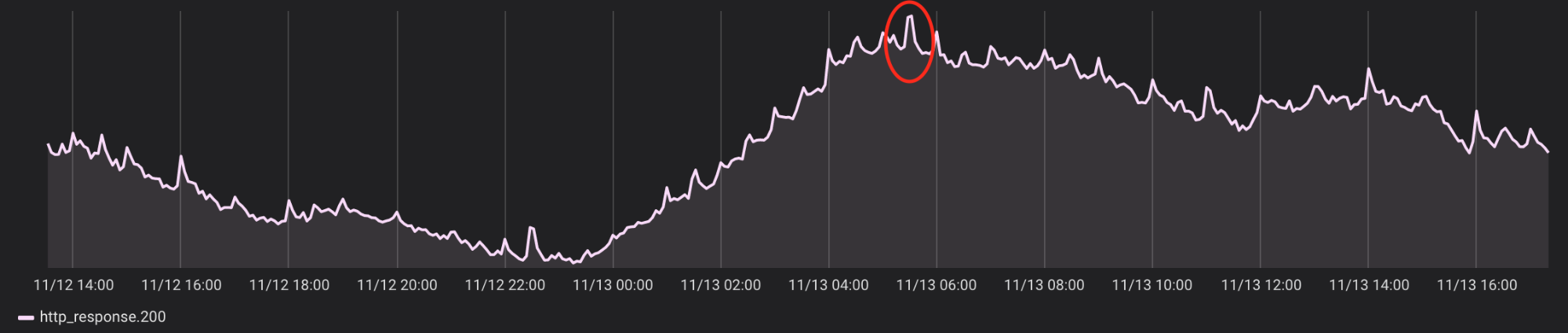
After assessing several downsampling algorithms, we decided to leverage the Largest Triangle Three Bucket (LTTB) algorithm for our use case. This algorithm does a good job of retaining the original shape of the data, including displaying outliers which are often lost with more naive methods, as well as possessing the useful property of only returning data points that exist in the original dataset. In Figures 7, 8, and 9, below, we demonstrate the differences between not downsampling (Figure 7), using a naive averaging algorithm (Figure 8), and using the LTTB algorithm (Figure 9):

Before developing M3QL, our metrics system only supported Graphite, a path-based language (e.g., foo.bar.baz). However, Graphite was not expressive enough for our needs, and we wanted a tag-based solution (e.g., foo:bar biz:baz) to make querying much simpler. More specifically, we wanted a solution that would improve discoverability and ease-of-use given the massive scale of our metrics storage.

In our experience, it is much more difficult to retrieve metrics using a path-based solution because the user must know exactly what each node represents in the metric. On the other hand, with a tag-based approach, there is no guessing, and auto-complete works much better. In addition to creating a tag-based query language, we also decided to make M3QL a pipe-based language (like UNIX) as opposed to a SQL-like language such as IFQL, or a C expression-like language such as PromQL. Pipe-based languages allow users to read queries from left to right as opposed to inside out. We break down a typical M3QL query showing failure rate of a certain endpoint in Figure 10, below:

It was a clear decision for us to integrate our query engine with Prometheus, a widely used open source monitoring system. Prometheus’s exporters, such as its node exporter, make it incredibly easy to retrieve hardware and kernel-related metrics.

On top of this, we found that many engineers have prior experience using PromQL, making it easier to onboard teams to M3. Since our query engine now natively supports PromQL, users do not need to learn additional languages nor will they need to recreate dashboards for third-party exporters. We also built the query engine’s API so that users can plug right into Grafana by selecting the Prometheus data source type.

As we continue building out the M3 ecosystem, we are committed to improving our query engine by adding new functionalities and tackling additional use cases.

Alerting and metrics go hand-in-hand, which is why alerting has been a top priority for us. We currently support running Grafana on our query engine. Internally, we run a more advanced closed source alerting application which we intend to open source in the coming months.  

Given Uber’s massive growth, we need to take into account both short, everyday queries and longer running ones for capacity planning and other summary/reporting use cases that often need data from multiple data sources. To support this, we plan to create a Presto connector, enabling users to run longer queries as well as make combining data from other data sources like SQL or HDFS possible.  

Try out the M3 query engine for yourself! Please submit pull requests, issues, and proposals to M3’s proposal repository.  

We hope you’ll get started with M3 and give us your feedback!

If you’re interested in tackling infrastructure challenges at scale, consider applying for a role at Uber.

Visit Uber’s official open source page for more information about M3 and other projects.