Modeling Censored Time-to-Event Data Using Pyro, an Open Source Probabilistic Programming Language
February 15, 2019 / Global
Time-to-event modeling is critical to better understanding various dimensions of the user experience. By leveraging censored time-to-event data (data involving time intervals where some of those time intervals may extend beyond when data is analyzed), companies can gain insights on pain points in the consumer lifecycle to enhance a user’s overall experience. Despite its prevalence, censored time-to-event data is often overlooked, leading to dramatically biased predictions.
At Uber, we are interested in investigating the time it takes for a rider to make a second trip after their first trip on the platform. Many of our riders engage with Uber for the first time through referrals or promotions. Their second ride is a critical indicator that riders are finding value in using the platform and are willing to engage with us in the long term. However, modeling the time to second ride is tricky. For example, some riders just don’t ride as often. When we analyze this time-to-event data before such a rider’s second ride, we consider their data censored.
Similar situations exist at other companies and across industries. For example, suppose that an ecommerce site is interested in the recurring purchase pattern of customers. However, due to the diverse pattern of customer behavior, the company might not be able to observe all recurring purchases for all customers, resulting in censored data.
In another example, suppose that an advertising company is interested in the recurring ad clicking behavior of its users. Due to the distinct interests of each user, the company might not be able to observe all clicks made by their customers. Users might not have clicked the ads until after the study concludes. This will result in censored time to next click data.
In modeling censored time-to-event data, for each individual of interest indexed by ![]() , we might observe data in the following form:
, we might observe data in the following form:
![]()
Here,![]() is the censorship label;
is the censorship label;![]() if the event of interest is observed; and
if the event of interest is observed; and![]() if the event of interest is censored. When
if the event of interest is censored. When![]() ,
, ![]() denotes the time-to-event of interest. When
denotes the time-to-event of interest. When ![]() ,
,![]() denotes the length of time until censorship happens.
denotes the length of time until censorship happens.
Let’s continue with the time-to-second ride example at Uber: if a rider took a second ride 12 days after their first ride, this observation is recorded as![]() . In another case, a rider took a first ride, 60 days have passed, and they have not yet returned to the app to take a second ride by a given cut-off date. This observation is recorded as
. In another case, a rider took a first ride, 60 days have passed, and they have not yet returned to the app to take a second ride by a given cut-off date. This observation is recorded as ![]() . The situation is illustrated in the picture, below:
. The situation is illustrated in the picture, below:

There is an ocean of survival analysis literature and over a century of statistical research has already been done in this area; much of which can be simplified using the framework of probabilistic programming. In this article, we walk through how to use the Pyro probabilistic programming language to model censored time-to-event data.
Relationship with churn modeling
Before proceeding, it’s worth mentioning that many practitioners in industry circumvent this censored time-to-event data challenge by setting artificially defined labels as “churn.” For example, an ecommerce company might define a customer as “churned” if they have not yet returned to the site to make another purchase in the past 40 days.
Churn modeling enables practitioners to massage observations into a classical binary classification pattern. As a result, churn modeling becomes very straightforward with off-the-shelf tools like scikit-learn and XGBoost. For example, the above two riders would be labeled into “not churned” and “churned,” respectively.
While churn modeling admittedly works in certain situations, it does not necessarily work for Uber. For example, some riders might only use Uber when they are on a business trip. If this hypothetical rider takes a trip for work every six months, we might end up mislabeling this business rider as having churned. As a result, the conclusion that we draw from a churn model might be misleading.
We are also interested in making interpretations from these models to elucidate the contribution of different factors to the user behavior observed. As a result, the model should not be a black box. We would love to have the capability to open up the model and make more informed business decisions with it.
To accomplish this, we can leverage, Pyro, a flexible and expressive open source tool for probabilistic programming.
Pyro for statistical modeling
Created at Uber, Pyro is a universal probabilistic programming language written in Python, built on the PyTorch library for tensor computations.
If you come from a statistics background with minimum Bayesian modeling knowledge or if you have been tinkering with deep learning tools like TensorFlow or PyTorch, you are in luck.
The following table summarizes some of the most popular projects for probabilistic programming:
| Software | BUGS / JAGS [1] | STAN | PyMC | TensorFlow Probability [4] | Pyro |
| Coding language | Domain Specific Language [2] | Domain Specific Language | Python | Python | Python |
| Underlying computational engine | Self | STAN Math Library | Theano [3] | TensorFlow [5] | PyTorch [6] |
Below, we highlight some key features about these different software projects:
- BUGS / JAGS are early examples of what came to be known as probabilistic programming. They have been under active development and usage for more than two decades in the statistical field.
- However, BUGS / JAGS are designed and developed mostly from the ground up. As a result, model specification is done using their domain specific language. Moreover, probabilistic programmers invoke BUGS / JAGS from wrappers in R and MATLAB. Users have to switch back and forth between coding languages and files, which is a bit inconvenient.
- PyMC relies on a Theano backend. However the Theano project was recently discontinued.
- TensorFlow Probability (TFP) originally started as a project called Edward. The Edward project was rolled into the TFP project.
- TFP uses TensorFlow as its computation engine. As a result, it supports only static computational graphs.
- Pyro uses PyTorch as computation engine. As a result, it supports dynamic computational graphs. This enables users to specify models that are diverse in terms of dataflow and is very flexible.
In short, Pyro is positioned at the very beneficial intersection of the most powerful deep learning tool chains (PyTorch) while standing on the shoulders of decades of statistical research. The result is an immensely concise and powerful, yet flexible probabilistic modeling language.
Modeling censored time-to-event data
Now, let’s jump into how we model censored time-to-event data. Thanks to Google Colab, users can check out extensive examples of the code and start modeling data without installing Pyro and PyTorch. You can even duplicate and play around with the workbook.
Model definition
For the purpose of this article, we define the time-to-event data as ![]() , with
, with![]() as the time-to-event and
as the time-to-event and![]() as the binary censoring label. We define the actual time-to-event as
as the binary censoring label. We define the actual time-to-event as![]() , which may not be observed. We define censoring time as
, which may not be observed. We define censoring time as ![]() , which for simplicity, we assume is a known fixed number. In summary, we can model this relationship as:
, which for simplicity, we assume is a known fixed number. In summary, we can model this relationship as:
![]()
![]()
We assume that![]() follows exponential distribution with scale parameter
follows exponential distribution with scale parameter ![]() , a variable dependent upon the following linear relationship with predictor of interest
, a variable dependent upon the following linear relationship with predictor of interest ![]() :
:
![]()
![]()
Here, ![]() is a softplus function, thereby ensuring that
is a softplus function, thereby ensuring that ![]() stays positive. Finally, we assume that
stays positive. Finally, we assume that![]() and
and![]() follow normal distribution as their prior distribution. For the purpose of this article, we are interested in evaluating the posterior distribution of
follow normal distribution as their prior distribution. For the purpose of this article, we are interested in evaluating the posterior distribution of![]() and
and![]() .
.
Generating artificial data
We first import all the necessary packages in Python:
To generate experiment data, we run the following lines:
Congratulations! You just ran your first Pyro function in the line with Note [1]. Here we drew samples from a normal distribution. Careful users might have noticed this intuitive operation is very similar to our workflow in Numpy.
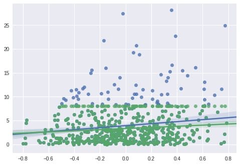
At the end of the above code block (Note 2), we generated a regression plot of ![]() (green),
(green), ![]() (blue) against
(blue) against ![]() , respectively. If we do not account for data censorship, we underestimate the slope of model.
, respectively. If we do not account for data censorship, we underestimate the slope of model.
Constructing models
With this fresh but censored data, we can begin constructing more accurate models. Let’s start with the model function, below:
In the code snippet above, we highlight the following notes to better clarify our example:
- Note 1: Overall, a model function is a process of describing how data are generated. This example model function tells how we generated y or truncation_label from input vector x.
- Note 2: We specify a prior distribution of
 and
and here and sample from them using the pyro.sample function. Pyro has a huge family of random distributions in the PyTorch project as well as in the Pyro project itself.
 - Note 3: We connect inputs
 ,
, , and
, and into
into vector denoted by variable link here.
 - Note 4: We specify the distribution of true time-to-event
 using exponential distribution with scale parameter vector link.
 - Note 5: For observation
 , if we observe the time-to-event data, then we contrast it with true observation y[i].
 - Note 6: If the data is censored for observation
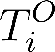
 , the truncation label (equalling to 1 here), follows Bernoulli distribution. The probability of seeing truncated data is the CDF of
 at point
 . We sample from the Bernoulli distribution and contrast it against real observation of truncation_label[i].
For more information on Bayesian modeling and using Pyro, check out our introductory tutorial.
Calculating inference using Hamiltonian Monte Carlo
Hamiltonian Monte Carlo (HMC) is a popular technique when it comes to calculating Bayesian inference. We estimate![]() and
and![]() using HMC, below:
using HMC, below:
The process above might take a long time to run. The slowness comes in great part due to the fact that we are evaluating the model through each observation sequentially. To speed up the model, we can vectorize using pyro.plate and pyro.mask, as demonstrated below:
In the code snippet above, we start by specifying the HMC kernel using the model specified. Then, we execute the MCMC against x, y, and the truncation_label. The MCMC sampled result object is next converted into an EmpiricalMarginal object that helps us to make inference along a_model parameter. Finally, we draw samples from posterior distribution and create a plot with our data, shown below:
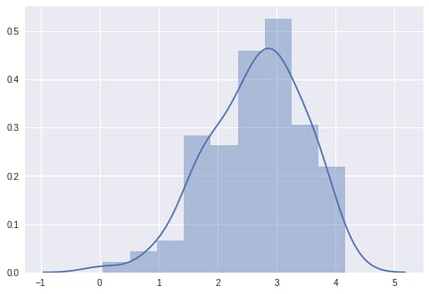
We can see that the samples are clustered around the real value of at 2.0.
Speeding up estimation using variational inference
Stochastic variational inference (SVI) is a great way to speed up Bayesian inference with large amounts of data. For now, it’s sufficient to proceed with the knowledge that a guide function is an approximation of the desired posterior distribution. The specification of a guide function can dramatically speed up the estimation of parameters. To enable stochastic variational inference, we define a guide function as:
guide = AutoMultivariateNormal(model)
By using a guide function, we can approximate the posterior distributions of parameters![]() and
and![]() as normal distributions, where their location and scale parameters are specified by internal parameters, respectively.
as normal distributions, where their location and scale parameters are specified by internal parameters, respectively.
Training the model and inferring results
The model training process with Pyro is akin to standard iterative optimization in deep learning. Below, we specify the SVI trainer and iterate through optimization steps:
If everything goes according to plan, we can see the print out of the above execution. In this example, we received the following results, whose means are very close to the true value of and specified:
a_model = 0.009999999776482582, b_model = 0.009999999776482582
a_model = 0.8184720873832703, b_model = 2.8127853870391846
a_model = 1.3366154432296753, b_model = 3.5597035884857178
a_model = 1.7028049230575562, b_model = 3.860581874847412
a_model = 1.9031578302383423, b_model = 3.9552347660064697
final result:
median a_model = 1.9155923128128052
median b_model = 3.9299516677856445
We can also check if the model has converged through the below code and arrive at Figure 3, below:
sns.plt.plot(losses)
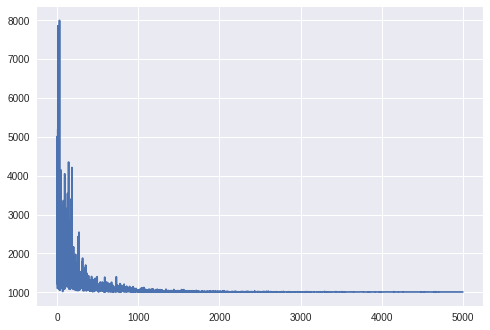
We can plot approximate posterior distribution using the guide.quantiles() function:
We can see that the guide functions center on the actual value of![]() and
and![]() , respectively below:
, respectively below:
Moving forward
We hope you leverage Pyro for your own censored time-to-event data modeling. To get started with the open source software, check out the official Pyro website for additional examples including an introductory tutorial and sandbox repository.
In future articles, we intend to discuss how you can leverage additional features of Pyro to speed up SVI computation, including using the plate api to batch process on samples of similar shape.
Interested in working on Pyro and other projects from Uber AI? Consider applying for a role on our team!

Hesen Peng
Hesen Peng is a senior data scientist at Uber’s Rider Data Science team.

Fritz Obermeyer
Fritz is a research engineer at Uber AI focusing on probabilistic programming. He is the engineering lead for the Pyro team.
Posted by Hesen Peng, Fritz Obermeyer
Related articles
Most popular

Introducing the Prompt Engineering Toolkit

Serving Millions of Apache Pinot™ Queries with Neutrino

Your guide to NJ TRANSIT’s Access Link Riders’ Choice Pilot 2.0

Connecting communities: how Harrisburg University expands transportation access with Uber
Products
Company


