Get a ride at the tap of a button; it’s as simple as transportation gets. But what looks simple on Uber’s frontend actually consists of complex architecture and services on the backend, including sophisticated routing and matching algorithms that direct cars to people and people to places. From the time you open the Uber app to the time you get dropped off, our routing engine is hard at work.
Here’s the history of solving routing problems at Uber, and how engineering has enabled us to evolve from several UberBLACKs in San Francisco five years ago to delivering millions of rides around the world every day.
The Beginning: 2011 – 2014
The estimated time of arrival (ETA) was one of our first features when the Uber platform started operating just over five years ago. It’s the first thing a rider sees when opening the app.

In Uber��’s early days, we used a combination of routing engines (including OSRM) to produce an ETA. (We didn’t have in-app navigation at this point, so we only used it for the ETA and map matching to display vehicle locations.)
We called this service “Goldeta”, which was essentially a model that sat on top of the routing engines and made an adjustment to those original estimates using our own historical Uber Data of similar routes in time and space. This solution, which ultimately took into account hundreds of thousands of Uber trips, compared them to the initial routing engine ETA. Goldeta worked better than using any single ETA alone. However, one issue with this approach was the cold start problem: when we launch in new cities we didn’t have enough data to inform an ETA offset (for new cities, our ETA used to be less accurate than older cities for precisely this reason). Also, as we grew we periodically needed to add new features whose development was slowed by having to implement it to an open source solution (OSRM) which wasn’t built from the ground up with a dispatching system in mind.
How to Build Your Own Routing Engine: A Primer
Goldeta served us well for a time, but as we grew to more cities and services (such as UberRUSH, launched in March 2014, and uberPOOL which we began work on in late spring 2014), it became clear that we needed a dedicated, in-house routing engine built for Uber. So in 2014 we began working on our own all-in-one routing engine, Gurafu. Gurafu’s goal? High-performance, highly-accurate ETA calculation specifically for Uber.
Before we launch into specifics, let’s discuss the essence of what you need in a routing engine. The whole road network is modeled as a graph. Nodes represent intersections, and edges represent road segments. The edge weights represent a metric of interest: often either the road segment distance or the time take it takes to travel through it. Concepts such as one-way streets, turn restrictions, turn costs, and speed limits are modeled in the graph as well.
Of course that isn’t the only way to model the real world. Some people want to model road segments as nodes, and edges as the transition between one road segment to another. This is called edge-based representation, in contrast to the node-based representation mentioned before. Each representation has its own tradeoffs, so it’s important to know what you need before committing to one or the other.
Once you have decided on the data structure, you can use different routing algorithms to find a route. One simple example you can try at home is the Dijkstra�’s search algorithm, which has become the foundation for most modern routing algorithms today. However, in a production environment, Dijkstra, or any other algorithm that works on top of an unprocessed graph, is usually too slow.
OSRM is based on contraction hierarchies. Systems based on contraction hierarchies achieve fast performance — taking just a few milliseconds to compute a route — by preprocessing the routing graph. (Below 100 milliseconds in the 99th percentile response time. We need this because this calculation is done every time before a vehicle is dispatched to a ride request.) But because the preprocessing step is very slow, it’s very difficult to make real-time traffic work. With our data, it takes roughly 12 hours to build the contracted graph using all the roads of the world, meaning we can never take into account up-to-date traffic information.
This is the reason some preprocessing and tweaking are often needed to speed up querying. (Recent examples of this class of algorithms in the literature include highway hierarchies, the ALT-algorithm, and customizable route planning.)
Here’s what we tried as we attempted to build our own routing engine starting in 2014:
1. Making Contraction Hierarchies Dynamic
In our routing graph, as new traffic information comes in, we need to be able to dynamically update those graph edge weights. As we mentioned, we used OSRM which uses contraction hierarchies as its routing algorithm. One drawback of contraction hierarchies is when edge weights are updated, the pre-processing step needs to be re-run for the whole graph, which could take a few hours for a big graph, for example one that covers the whole planet. This makes contraction hierarchies unsuitable for real-time traffic updates.
Contraction hierarchies’ preprocessing step can be significantly faster by doing dynamic updates, where the ordering of the nodes remains the same and only the edges that change due to traffic are updated. This decreases the precomputation significantly. With this approach, it takes just 10 minutes to do a dynamic update of the world graph even with 10% of the road segments changing traffic speed. However, 10 minutes is still too much of a delay for the traffic update to finally be considered for ETAs. So, this path was ultimately a dead end.
2. Sharding
We can also break up the graphs into geographic regions, aka sharding. Sharding speeds up the time it takes to build the contracted graph. However, this requires quite a bit of engineering on our infrastructure for it to work, and would introduce bottlenecks in the cluster size of servers for each region. If one region received too many requests during peak hours, the other servers couldn’t share the load. We wanted to make the most out of the limited numbers of servers we had, so we did not implement this solution either.
3. A* Algorithm
For real-time updates and in a small scale, we tried the A* search algorithm. At a high level, A* is Dijkstra’s search algorithm with heuristics, so A* prioritizes whichever nodes are most likely to find a route from A to B. This means we can update the edge weights of the graph in real-time to account for traffic conditions without needing to do any precomputation. And since most routes we need to calculate are for short trips (the en route time from drivers to riders), A* works well in those situations.
But we knew A* was a temporary solution because it’s really slow for long routes: the A* response grows geometrically in relation to the depth of nodes traversed. (For example, the response time for a route from the Presidio to the Mission District in San Francisco is ~120 milliseconds, several times longer than contraction hierarchies.)
Even A* with landmarks, which makes use of the triangle inequality and several pre-computation tricks, does not increase the time of A* traversal enough to make it a viable solution.
For long distance trips, A* simply doesn’t have a quick enough response time, so we end up falling back to using a contracted graph that doesn’t have the dynamic edge weights to begin with.
2015 and Beyond
We needed the best of both worlds: we needed precomputation to make it fast, and the ability to update edge weights quickly enough to support real-time traffic. Our solution effectively handles real-time traffic updates by re-running the preprocessing step only for a small part of the whole graph. Since our solution divides the graph into layers of small cells which are relatively independent of each other, the preprocessing step is run in parallel when needed to make it even faster. (To find out more, click here!)
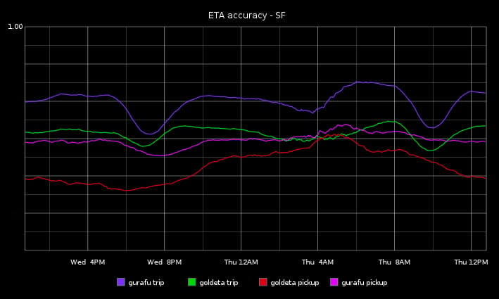
To understand the improvements we’ve made before we pushed our new routing engine fully live, we tracked what the real-time ETA accuracy between Gurafu and Goldeta was in January 2015 once our first Gurafu version was ready for testing:

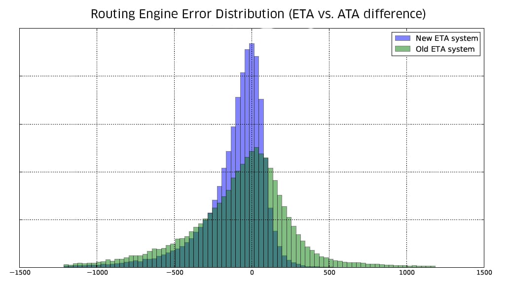
In April 2015, we globally launched our new routing engine which allowed us to have a more accurate ETA prediction system. The new system is based on Gurafu, our new routing engine, and Flux, Uber’s first historical traffic system based on GPS data we collect from partner phones. We used our in-house ETA system primarily for pickups, but we’ve also been tracking ETA accuracy for full trip length ETAs.
To measure ETA accuracy, we built a tool which would ingest our Kafka logs in real time to retrieve the actual time of arrival (ATA), and compare that to our ETA. Additionally, our team members may report ETA bugs directly from the app. Measuring route quality sometimes requires visual inspection on a case-by-case basis, so we also built a rich set of web tools to visualize, inspect and compare routes from different models and providers.

These sanity checks show we’ve come a long way in the last year.
Ultra-efficient route planning and highly accurate ETAs are critical. We use modern routing algorithms to build a carefully optimized system capable of handling hundreds of thousands of ETA requests per second, with single-digit milliseconds response time. All of our new services, such as uberPOOL and UberEATS start with this system.
This journey is not over. The importance of accuracy and efficiency to contextually determine the best way to get somewhere, and when, will continue to rise as we expand and improve products like uberPOOL and beyond. We’re going to make phoning home even more reliable and intelligent. If this sounds like a challenge you’re interested in, we’d love for you to join us.
Posted by Thi Nguyen